Traffic Forecasting with BigQuery ML in DBT using GA4 Data

We are going to use the BigQuery ML Arima Plus model, using the dbt_ml package, to create a daily forecast of traffic. We will use GA4 data from the raw, BigQuery export processed through the dbt-GA4 package as the data source for these traffic forecasts.

BigQuery ML simplifies the creation and running of machine learning models using SQL. DBT simplifies the management and deployment of SQL transformations, but it does so in a warehouse-agnostic way so niche features unique to one particular warehouse are unlikely to be supported.

Enter the dbt package ecosystem and the dbt_ml package in particular which adds BigQuery ML support to dbt giving you a custom model type for training BigQuery ML models and custom macros for making forecasts and predictions of your trained models.

This post assumes as basic level of knowledge of dbt, and the dbt-GA4 package. If you are new to any of this, I recommend taking my free dbt-GA4 Setup course, which takes you far enough that you can work with the code in this post albeit slightly inefficiently, and the paid Advanced dbt-GA4 course which covers building optimized models that we would prefer to use with BigQuery ML.

What use are traffic forecasts?

Traffic forecasts are the sort of thing that everyone thinks that they want but really they’ll never use.

There are some situations where traffic forecasts can be quite compelling, though. In the publishing industry, the main source of revenue is usually direct ad sales. Publishers will sell x-number of ad impressions per month in a particular section of their site to interested advertisers. Leftover inventory goes to auction, but they make much less from auctioned inventory.

This creates a situation where the publishers are contractually obligated to provide a certain number of impressions often on a specific section of their site. Detecting shortfalls early means that the editorial team can take steps like commissioning extra articles to hit their numbers or the advertising team can start buying extra traffic earlier which is less expensive than buying that traffic over a short time-frame.

Additionally, publishers are incentivized to sell as much inventory as possible because they make so much more from direct sales than they do from auctioned inventory. Having a good forecasts helps sales people direct their efforts to sell inventory in sections of the site that are not yet fully subscribed.

What about forecasting ecommerce revenue?

You could certainly use this for forecasting ecommerce revenue. But I would highly recommend that you not use Google Analytics data for this and rather pull and model accounting or ERP data in your warehouse because that data is a lot less messy to begin with as it is not subject to the many web-data collection issues.

It may be of some use to forecast ecommerce revenue by acquisition channel, which you can’t do with ERP/accounting data, in which case there is some justification for using web data to forecast revenue, but this still isn’t a very compelling use for forecasts. What decisions does this kind of forecast support? Are you going to change your marketing investments based on this forecast? Maybe, but accounting and ERP data can be used for things like forecasting demand for individual SKUs so that you can optimize your inventory which provides a much more tangible return on your forecasting investment.

What is ARIMA

Use ARIMA for forecasting time series data. It stands for Autoregressive Integrated Moving Average.

ARIMA takes three parameters labeled ‘p’, ‘d’, and ‘q’.

The ‘p’, ‘d’, and ‘q’ values correspond respectively to ‘ar’, ‘i’, and ‘ma’ of ARIMA.

I need to warn everyone here that my statistics abilities are weak. I might use some language wrong while trying to simplify the concepts. Please forgive and share any corrections in the comments.

Autoregressive, the ‘ar’ in ARIMA, is a prediction based on a previous value. The ‘p’ value is the lag period which represents the number of previous data points you use in your prediction.

Because we will be working with daily data, p=1 means that we will use yesterday’s data to predict today and p=2 uses the last two days.

The optimal ‘p’ parameter is usually chosen by data analysis using ACF or PACF plots.

Integrated, the ‘i’ in ARIMA, means that the data is what is known as stationary. Stationarity means that the mean, variance, and autocorrelation of the data do not change over time.

You use the ‘d’ parameter to difference the data to make it stationary removing trends.

If your traffic is flat, then d = 0 would be appropriate.

If there’s a clear upward trend, then d = 1 would be appropriate.

The ‘d’ parameter handle trends. You should fix noise, like double-counting traffic due to tagging issues, before feeding the data in to ARIMA as ARIMA assumes that any noise present in the data is random. Non-random noise can lead to correlations that throw off the ARIMA prediction.

There are several techniques that you can use to test your data’s stationarity:

• Augmented Dickey-Fuller (ADF) Test
• Kwiatkowski-Phillips-Schmidt-Shin (KPSS) Test
• Phillips-Perron (PP) Test

You will need to run these tests in Python or R (or let Google do this with AUTO_ARIMA)

Moving average is the lagged forecast errors between observed and predicted data. ARIMA uses the data you give it to predict data that you already know the values for in order to calculate the typical error of the prediction and account for these errors when making predictions that you actually care about.

The ‘q’ parameter in an ARIMA model is the number of past forecast errors (lagged errors) from previous time steps that the model considers when making future predictions.

ARIMA in BigQuery ML

BigQuery ML does not use standard ARIMA but rather their own flavor of ARIMA called ARIMA_PLUS.

The main advantage of Google’s model is it adds a number of options that improve the quality of data that feeds in to ARIMA like seasonalities, holiday corrections, and automated parameter selection and readjusts the forecasts that come out of the model giving you better forecasts.

The documentation for the ARIMA_PLUS model in BigQuery ML lists an intimidating number of model options for people who are using BigQuery ML to dip in to machine learning.

model_option_list:
MODEL_TYPE = 'ARIMA_PLUS'
    [, TIME_SERIES_TIMESTAMP_COL = string_value ]
    [, TIME_SERIES_DATA_COL = string_value ]
    [, TIME_SERIES_ID_COL = { string_value | string_array } ]
    [, HORIZON = int64_value ]
    [, AUTO_ARIMA = { TRUE | FALSE } ]
    [, AUTO_ARIMA_MAX_ORDER = int64_value ]
    [, AUTO_ARIMA_MIN_ORDER = int64_value ]
    [, NON_SEASONAL_ORDER = (int64_value, int64_value, int64_value) ]
    [, DATA_FREQUENCY = { 'AUTO_FREQUENCY' | 'PER_MINUTE' | 'HOURLY' | 'DAILY' | 'WEEKLY' | 'MONTHLY' | 'QUARTERLY' | 'YEARLY' } ]
    [, INCLUDE_DRIFT = { TRUE | FALSE } ]
    [, HOLIDAY_REGION = string_value | string_array ]
    [, CLEAN_SPIKES_AND_DIPS = { TRUE | FALSE } ]
    [, ADJUST_STEP_CHANGES = { TRUE | FALSE } ]
    [, TIME_SERIES_LENGTH_FRACTION = float64_value ]
    [, MIN_TIME_SERIES_LENGTH = int64_value ]
    [, MAX_TIME_SERIES_LENGTH = int64_value ]
    [, TREND_SMOOTHING_WINDOW_SIZE = int64_value ]
    [, DECOMPOSE_TIME_SERIES = { TRUE | FALSE } ]
    [, FORECAST_LIMIT_LOWER_BOUND = float64_value ]
    [, FORECAST_LIMIT_UPPER_BOUND = float64_value ]
    [, SEASONALITIES = string_array ]
    [, HIERARCHICAL_TIME_SERIES_COLS = {string_array } ]
    [, KMS_KEY_NAME = string_value ]

Technically, you don’t need most of these, but they actually make it easier to work with ARIMA so lets look at a few of them.

AUTO_ARIMA and NON_SEASONAL_ORDER

You need to set one of AUTO_ARIMA or NON_SEASONAL_ORDER as these are the options that tell ARIMA how to process the data.

For those of you who can’t be bothered to understand these values, just set AUTO_ARIMA = TRUE. This lets BigQuery ML decide which values are best here.

Otherwise, you need to set ‘p’, ‘d’, and ‘q’ values and this is done via the NON_SEASONAL_ORDER = (p, d, q) option where p and q are values between 0 and 5 and d is between 0 and 2.

TIME_SERIES_TIMESTAMP_COL and TIME_SERIES_DATA_COL

Minimally, you need to set AUTO_ARIMA = TRUE and pass TIME_SERIES_TIMESTAMP_COL and TIME_SERIES_DATA_COL to ARIMA_PLUS which are, respectively, the date or timestamp column for the time dimension and the metric that you want to predict.

HORIZON, SEASONALITIES and DATA_FREQUENCY

These are three important parameters that are easy to understand.

The DATA_FREQUENCY is the grain of the data.

Since we’re looking for daily forecasts, it will be daily DATA_FREQUENCY = 'DAILY.

The HORIZON is how many values to predict. Since we’re working with daily totals, it is how many days of data to predict. It defaults to 1000 which is way more than you should ever need when predicting traffic, so it is almost a requirement.

And SEASONALITIES is the length of a cycle.

With daily web data it should be usually be weekly and yearly SEASONALITIES = ('WEEKLY', 'YEARLY') as most sites get traffic dips on weekends and various annual trends like slightly lower summer traffic and a big dip on Christmas day (or various other holidays depending on the country).

The dbt_ml package

The dbt_ml package includes a custom dbt models for deploying BigQuery ML. Using this package, you set the various BigQuery ML parameters using a special materialization and ml_config block within your model config block.

Using BigQuery ML is a two-step process: first you train your model, and then you predict or forecast. The dbt_ml package inclues a special materialization that interacts with an ml_config block within your model config block for training and a series of selection macros for forecasting and predicting.

In the case of ARIMA_PLUS, you use the forecasting macro.

Predicting daily total traffic

In the Advanced dbt-GA4 course, we created a daily summary table called agg_ga4__daily to make reporting top-level summary metrics, and year-to-date and 13-month trend sparklines fast and inexpensive to report. This is our maximally optimized model for daily data and it’s what we should use to forecast daily traffic.

Training the model

With the dbt_ml package installed in your dbt project, you would train your model for the next 60 days for a North American site using the following dbt model:

tr_arima__page_views

{{
    config(
        materialized='model',
        ml_config={
            'model_type': 'arima_plus',
            'time_series_timestamp_col': 'date',
            'time_series_data_col': 'page_views',
            'horizon': 60,
            'auto_arima': true,
            'data_frequency': 'daily',
            'holiday_region': 'NA',
            'seasonalities' : ['weekly','yearly']
        }
    )
}}

select 
    date,
    page_views
from {{ref("agg_ga4__daily")}}
where date < current_date

Let’s break that down a little.

The materialized line tells dbt to use the custom materialization from the dbt_ml package.

materialized='model',

The ml_config block tells dbt_ml what model to use.

'model_type': 'arima_plus',

Which inputs to use as your time column and the column of data you want to run your prediction on. Note that time_series_timestamp_col can be a date-type column and does not have to be a timestamp despite the name.

'time_series_timestamp_col': 'date',
'time_series_data_col': 'page_views',

The remaining ml_config values are taken directly from the model_option_list parameters for ARIMA_PLUS:

'horizon': 60,
'auto_arima': true,
'data_frequency': 'daily',
'holiday_region': 'NA',
'seasonalities' : ['weekly','yearly']

In this case, we’re predicting the next 60 days of data, using auto_arima with daily data in North America that displays weekly and yearly seasonal patterns.

The select statement pulls the data that we want to use and lets us do some light processing on the data (in this case, ensuring that we don’t feed today’s data in to the model since it is incomplete).

select 
    date,
    page_views
from {{ref("agg_ga4__daily")}}
where date < current_date

I put training models in an ml_train folder and also set that as my schema so that all of my training models are kept in the same dataset in BigQuery. Here’s the model config for my cj dbt project:

models:
  cj:
    ml_train:
      +schema: ml_train

Running dbt run --select tr_arima__page_views will create a Models folder in the designated dataset with new model named tr_arima__page_views:

You can get some information from the various tabs, but the interface really doesn’t include much that’s of use to any but machine learning experts.

You can see the actual code that was sent to BigQuery in the target/run/<project_name>/models/ml_train folder:

create or replace model `cj-data-warehouse`.`cj_ml_train`.`tr_arima__page_views`

options(
    model_type="arima_plus",
    time_series_timestamp_col="date",
    time_series_data_col="page_views",
    horizon=60,
    auto_arima=True,
    data_frequency="daily",
    holiday_region="NA",
    seasonalities=['weekly', 'yearly']
)as (

select 
    cast(date as timestamp) as date,
    page_views
from `cj-data-warehouse`.`cj_analytics`.`agg_ga4__daily`
where date < current_date
        );

Copying, pasting, and running this code in BigQuery would train the model again.

If you don’t have a daily aggregate table set up and instead want to use the page_view fact table that we created in the dbt-GA4 Setup course, then you can use exactly the same settings and just modify the select statement for model training.

select 
    cast(event_date_dt as timestamp) as date,
    count(*) as page_views
from {{ref("fct_ga4__event_page_view")}}
where event_date_dt < current_date
group by 1

Forecasting with the model

With the model trained, you now have to run your forecast. Most of the BigQuery ML models implemented in the dbt_ml package use the predict macro, but ARIMA_PLUS is one of the few that uses the forecast macro.

Forecasting or predicting data is as simple as calling the macro in your select statement.

I prefix my model names with fcast or prdct, depending on which macro is called, and add the model name as prefixes, so since ARIMA_PLUS uses forecast I prefix the name fcast_arima_. I like to put all of my forecasts and predictions in a single folder titled ml_predict and give it the same schema so that the forecasts and predictions appear in the same dataset in BigQuery.

models:
  cj:
    ml_predict:
      +schema: ml_predict

The actual forecast model is really simple. Here’s my page views forecast:

fcast_arima__page_views

{{
    config(
        materialized='table'
    )
}}

select * from {{ dbt_ml.forecast(ref('tr_arima__page_views')) }}

Running dbt run --select fcast_arima__page_views results in a new table containing your forecasts with the following schema:

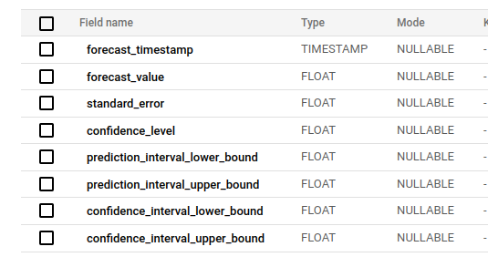
We are mainly interested in the forecast_timestamp which is the start of the day in UTC for the forecast and the forecast_value which contains the actual forecast.

Later on, we’re going to build a model on top of this to show how to use the forecast data and combine it with actual values and a target.

Predicting Daily Traffic by Channel

The ARIMA Plus model in BigQuery ML lets you use a parameter to predict multiple time series in a single query.

Training ARIMA with time_series_id_col

Just by setting the time_series_id_col parameter in the ml_config block and adding channel to your query, you can predict by channel and get a prediction by channel.

tr_arima__page_views_by_channel

{{
    config(
        materialized='model',
        ml_config={
            'model_type': 'arima_plus',
            'time_series_timestamp_col': 'date',
            'time_series_data_col': 'page_views',
            'time_series_id_col' : 'session_default_channel_grouping',
            'horizon': 60,
            'auto_arima': true,
            'data_frequency': 'daily',
            'holiday_region': 'NA',
            'seasonalities' : ['weekly','yearly']
        }
    )
}}
with dim as (
    select 
        session_partition_key 
        , session_partition_date
        , session_default_channel_grouping
    from {{ref('dim_ga4__sessions_daily')}}
    where session_partition_date < current_date
)
, fct as (
    select 
        d.session_partition_date as date 
        , d.session_default_channel_grouping 
        , sum(f.session_partition_count_page_views) as page_views
    from {{ref('fct_ga4__sessions_daily')}} as f 
    left join dim as d using(session_partition_key)
    group by 1,2
)
select * from fct 

The big difference in this query is that we’ve added the time_series_id_col parameter to ml_config.

'time_series_id_col' : 'session_default_channel_grouping'

We also get the data from the session fact and dimension tables as the page view count was in the fact table and the channel grouping was in the dimension table.

This could get quite expensive if you have a lot of sessions every day that go back a long time so you may want to create an aggregate table for attribution data similar to the daily aggregate table we created in the Advanced dbt-GA4 course.

Forecasting with time_series_id_col

Of course, we also need to do our forecasts.

fcast_arima__page_views_by_channel

{{
    config(
        materialized='table'
    )
}}

select * from {{ dbt_ml.forecast(ref('tr_arima__page_views_by_channel')) }}

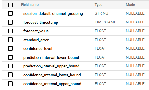
The resultant forecast includes the same columns as the example that didn’t set time_series_id_col but adds session_default_channel_grouping.

If we were to apply this to the publisher example from earlier where advertisers are buying ads on specific sections of the site, then the analytics implementation would need to pass a site_section or similar parameter to GA4 which would then need to be configured in dbt-GA4 and processed possibly in to an agg_ga4__site_sections model that is built from the fct_ga4__event_page_view model and includes the various metrics that you want to report on by site_section and date.

The dbt_ml model would look something this:

ml_arima__page_views_by_site_section

{{
    config(
        materialized='model',
        ml_config={
            'model_type': 'arima_plus',
            'time_series_timestamp_col': 'date',
            'time_series_data_col': 'page_views',
            'time_series_id_col' : 'site_section'
            'horizon': 60,
            'auto_arima': true,
            'data_frequency': 'daily',
            'holiday_region': 'NA',
            'seasonalities' : ['weekly','yearly']
        }
    )
}}

select 
    date
    , site_section
    , page_views
from {{ref("agg_ga4__site_sections")}}
where date < current_date

You might also then want to connect to the ad sales system and CRM so that you can combine this data with data on how many impressions have been sold for the month so that you can project which sections are going to hit the quota and which ones need help but that is beyond the scope of this article.

Using the Predictions in a Report

When pulling this data into a report, you’ll probably want to get the actual daily page views up to yesterday, and then the predicted daily page views from today until the end of the month (or whatever other period). Because we are predicting daily totals, we don’t want part of a day’s data so we get today’s data from the forecasts rather than actual numbers which shouldn’t be complete.

You can do this in you in your data visualization software, but it’s easier to do in BigQuery.

With the first daily totals example, we would run something like the following:

{{config(materialized='view')}}

with act as (
    select
        date 
        , page_views
    from {{ref('agg_ga4__daily')}}
    where date < current_date
    and date >= date_trunc(current_date, month)
)
, fore as (
    select
        extract(date from forecast_timestamp) as date
        , forecast_value as page_views 
    from {{ref('fcast_arima__page_views')}} 
    where extract(date from forecast_timestamp) >= current_date 
    and extract(date from forecast_timestamp) < date_trunc(date_add(current_date, interval 1 month), month)
    union all select * from act
)
, targ as (
    select
        300000 / count(fore.date) as daily_page_view_target
    from fore
)
select
    fore.date 
    , fore.page_views
    , targ.daily_page_view_target
from fore
cross join targ

Let’s break this down.

We get the month-to-date actual values up until yesterday.

with act as (
    select
        date 
        , page_views
    from {{ref('agg_ga4__daily')}}
    where date < current_date
    and date >= date_trunc(current_date, month)
)

We get the first day of this month with date_trunc(current_date, month).

Then we get the forecast values. BigQuery ML saves the ARIMA forecasts to a column titled forecast_value and we have to use forecast_timestamp to get the dates for today until the end of the month.

We calculate the first day of next month by adding a month to today’s date, extracted from the timestamp, truncating the date to the beginning of the month (which is the first of next month) and using the date is less than comparison to scrub out next month’s forecasts.

, fore as (
    select
        extract(date from forecast_timestamp) as date
        , forecast_value as page_views 
    from {{ref('fcast_arima__page_views')}} 
    where extract(date from forecast_timestamp) >= current_date 
    and extract(date from forecast_timestamp) < date_trunc(date_add(current_date, interval 1 month), month)
    union all select * from act
)

We get the forecasts from today forward on this line: where extract(date from forecast_timestamp) >= current_date.

And we limit that to forecast until the end of the month on this line: and extract(date from forecast_timestamp) < date_trunc(date_add(current_date, interval 1 month), month).

We convert the forecast_timestamp to a date value extract(date from forecast_timestamp) and make sure that it is less than the first day of the next month date_trunc(date_add(current_date, interval 1 month), month).

Then, we pull in our target number of page views for the end of the month. I’ve hard-coded this here, but you might get this from another system or a Google Sheet synced to BigQuery.

, targ as (
    select
        300000 / count(fore.date) as daily_page_view_target
    from fore
)

The count(fore.date) works because we’re only getting actual values from the start of the month to yesterday and forecast values from today until the end of the month, so a count of dates gives you the number of days in a month.

And, finally, we join the data.

select
    fore.date 
    , fore.page_views
    , targ.daily_page_view_target
from fore
cross join targ

I put the actuals and forecasts in the same column so that you can sum page_views when plotting on a line graph and see a continuous line that can be compared with a continuous line using the daily_target to see whether you are ahead or behind your monthly target.

Using ARIMA_PLUS for web data

Hopefully, this will help demystify BigQuery ML a little as the documentation can be a little intimidating.

The dbt_ml package simplifies the use of BigQuery ML a little but, if you inspect the code that you actually send to BigQuery in the target folder, you will see that the code is not particularly complex.

The main challenge is in understanding the available options and setting them correctly.

Traffic prediction for publishers with direct ad sales is a truly useful application of ARIMA_PLUS, but I would be careful about offering forecasts in most other situations as the stakeholders will almost certainly think that they want it but they will almost never use it in practice making the forecast a distraction at best.